QuTiP Notes 1
Useful qutip tutorials:
Basics
Introduction to QuTiPSuperoperators, Pauli basis and channel contraction
Visualization
Wigner functions
Quantum mechanics lectures with QuTiP
Jaynes-Cummings modelCavity-qubit gateskey: time dependent Hamiltonian strength
cQED in the dispersive regimeSuperconducting charge qubitsGallery of Wigner functions
Optimal control
OverviewGRAPE (GRadient Ascent Pulse Engineering)
second order gradient ascent
HadamardQFTLindbladianSymplectic
~first order gradient ascent~
~CNOT (2017)~ 1 hour
~iSWAP (2017)~ 20 s
~Single-qubit rotation (2017)~ 1 min
~Toffoli gate (2017)~ 20 hours
CRAB (Chopped RAndom Basis)
QFT (CRAB)~State to state (CRAB)~
%matplotlib inline
import numpy as np
import matplotlib.pyplot as plt
import matplotlib as mpl
from qutip import *
Introduction to QuTiP
State vectors, Density matrices, Operators
Hermitian: \(A^{\dagger}=A\)
# basis(2,1), fock(2,1), coherent(N=2,alpha=1)
# fock_dm(2,1), coherent_dm(2,1), thermal_dm(2,1)
# sigmax(), sigmay(), sigmaz()
a = destroy(2)
create(2)
x =       (a + a.dag())/np.sqrt(2)
p = -1j * (a - a.dag())/np.sqrt(2)
Composite systems & Jaynes-Cummings model
Jaynes-Cumming model:
Rotating-wave approximation:
def Hjc(dimC,omegaC,omegaA,g,rotWavApprox=False):
    a = tensor(destroy(dimC),qeye(2))
    sm = tensor(qeye(dimC),destroy(2))
    if rotWavApprox: inte = g * ( a*sm.dag() + a.dag()*sm )
    else: inte = g * (a+a.dag()) * (sm+sm.dag())
    return inte + omegaC*a.dag()*a \
        -0.5*omegaA*tensor(qeye(dimC),sigmaz())
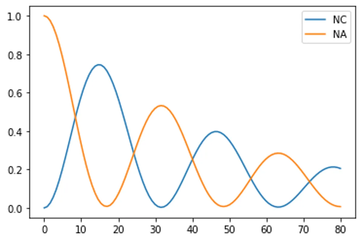
Unitary dynamics
Note mesolve returns either result.expect (when e_ops is
not empty) or result.states, but not both
def plot(result,labels=None):
    numExpect = len(result.expect)
    for i in range(numExpect):
        label = i if labels is None else labels[i]
        plt.plot(t, result.expect[i], label=label)
    plt.legend(); plt.show()


dimC = 4
t = np.linspace(0, 80, 100)
H = Hjc(dimC,1,1,0.1)
psi0 = tensor(fock(dimC,0),fock(2,1))
# find expectation for
X = tensor(qeye(dimC),sigmax())
Z = tensor(qeye(dimC),sigmaz())
aC = tensor(destroy(dimC),qeye(2))
NC = aC.dag() * aC
aA = tensor(qeye(dimC),destroy(2))
NA = aA.dag() * aA
# collapse operators
C1 = 0.2*aC
result = mesolve(H, psi0, t, [C1], [NC,NA])
plot(result,['NC','NA'])
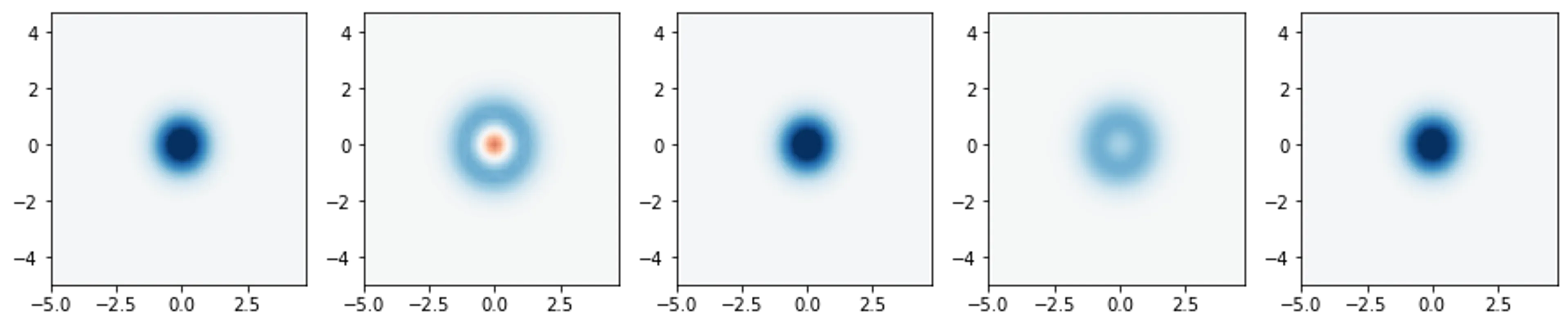
Wigner functions
def plotWigner(rhoList):
    figGrid = (2, len(rhoList)*2)
    fig = plt.figure(figsize=(2.5*len(rhoList),5))
    x = np.arange(-5, 5, 0.25)
    for idx, rho in enumerate(rhoList):
        W = wigner(rho, x, x)
        ax = plt.subplot2grid(figGrid, (0, 2*idx), colspan=2)
        ax.contourf(x, x, W, 100, norm=mpl.colors.Normalize(-.25,.25), cmap=plt.get_cmap('RdBu'))
    plt.tight_layout()
    plt.show()


result = mesolve(H, psi0, t, [C1], [])
def getRhoCavity(n): return ptrace(result.states[n], 0)
rhoList = list(map(getRhoCavity,np.arange(0,100,20)))
plotWigner(rhoList)
Cavity-qubit gates
def fToOmega(f): return 2*np.pi*f


dimC = 4
t = np.linspace(0, 100, 500)
aC = tensor(destroy(dimC),qeye(2),qeye(2))
aQ1 = tensor(qeye(dimC),destroy(2),qeye(2))
aQ2 = tensor(qeye(dimC),qeye(2),destroy(2))
NC  = aC.dag()  * aC
NQ1 = aQ1.dag() * aQ1
NQ2 = aQ2.dag() * aQ2

ZQ1 = tensor(qeye(dimC),sigmaz(),qeye(2))
ZQ2 = tensor(qeye(dimC),qeye(2),sigmaz())

g1 = fToOmega(0.01)
g2 = fToOmega(0.0125)
HCQ1 = g1 * (aC.dag() * aQ1 + aC * aQ1.dag())
HCQ2 = g2 * (aC.dag() * aQ2 + aC * aQ2.dag())

omegaC0 = fToOmega(5)
omegaQ10 = fToOmega(3)
omegaQ20 = fToOmega(2)
t0Q1 = 20
TQ1 = (1*np.pi)/(4 * g1)
t0Q2 = 60
TQ2 = (2*np.pi)/(4 * g2)

def step(t,t0,h1,h2,w=None):
    return h1+(h2-h1)*(t>t0)
def omegaC(t,args=None):
    return omegaC0
def omegaQ1(t,args=None):
    h2 = omegaC0 - omegaQ10
    return omegaQ10 + step(t,t0Q1,0,h2) - step(t,t0Q1+TQ1,0,h2)
def omegaQ2(t,args=None):
    h2 = omegaC0 - omegaQ20
    return omegaQ20 + step(t,t0Q2,0,h2) - step(t,t0Q2+TQ2,0,h2)

Ht = [ [NC,omegaC], [-0.5*ZQ1,omegaQ1], [-0.5*ZQ2,omegaQ2],
       HCQ1+HCQ2 ]
psi0 = tensor(fock(dimC,0),fock(2,1),fock(2,0))
result = mesolve(Ht,psi0,t,[],[NC,NQ1,NQ2])
plot(result,['NC','NQ1','NQ2'])

result = mesolve(Ht,psi0,t,[],[])
rhoQubits = ptrace(result.states[-1], [1,2])

from qutip.qip.operations import phasegate,sqrtiswap
rhoQubitsIdeal = ket2dm(
    tensor(phasegate(0), phasegate(-np.pi/2))
    * sqrtiswap()
    * tensor(fock(2,1),fock(2,0))
)

fidelity(rhoQubits,rhoQubitsIdeal), \
concurrence(rhoQubits)
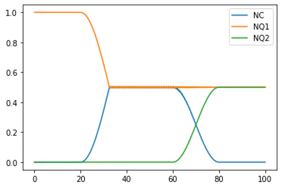
(0.01969740679409353, 0.9999376665389423)
cQED in the dispersive regime
qubit-resonator system
\[\displaystyle H = \omega_r a^\dagger a - \frac{1}{2} \omega_q \sigma_z + g (a^\dagger + a) \sigma_x\]\(g\) : dipole interaction strength
\(\Delta = |\omega_r-\omega_q|\) : detuning
\(\Delta \gg g\) : dispersive regime
Dispersive regime: effective Hamiltonian
\[\displaystyle H_{\text{eff}} = \omega_r a^\dagger a - \frac{1}{2}\omega_q \sigma_z + \underbrace{\chi}_{g^2/\Delta} (a^\dagger a + 1/2) \sigma_z\]The dispersive regime can be used to resolve the photon number states of a microwave resonator by monitoring a qubit that was coupled to the resonator.
Two-operator two-time correlation function
\[\left<A(t+\tau)B(t)\right>\]
dimC = 20
omegaC = fToOmega(2)
omegaQ = fToOmega(3)
chi = fToOmega(0.025)
aC = tensor(destroy(dimC),qeye(2))
aQ = tensor(qeye(dimC),destroy(2))
NC = aC.dag()*aC
NQ = aQ.dag()*aQ
xC = aC.dag()+aC
xQ = aQ.dag()+aQ
ZQ = tensor(qeye(dimC),sigmaz())
XQ = tensor(qeye(dimC),sigmax())
I = tensor(qeye(dimC),qeye(2))
# something is wrong with the tutorial ?
# H = omegaC*NC - 0.5*omegaQ*ZQ + chi*(NC+0.5*I)*ZQ
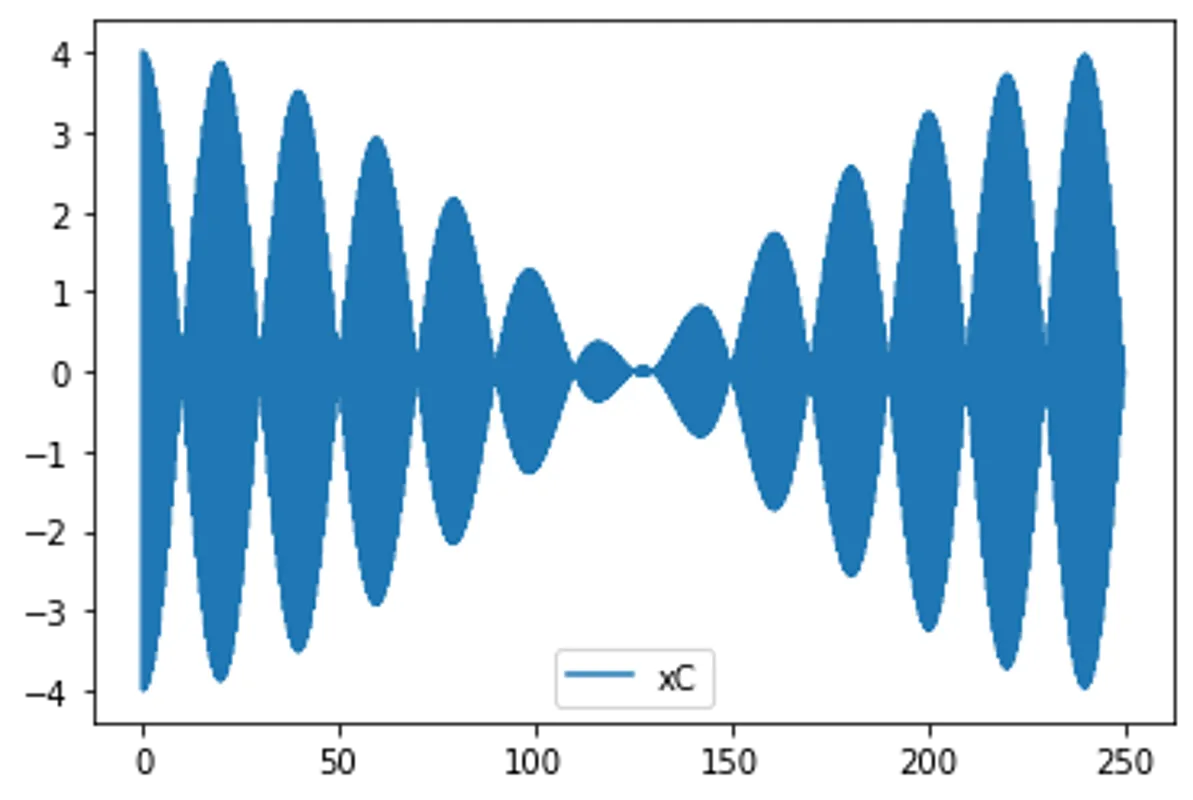
H = omegaC*(NC+0.5*I) + 0.5*omegaQ*ZQ + chi*(NC+0.5*I)*ZQ
psi0 = tensor( coherent(dimC,np.sqrt(4)),
(fock(2,0)+fock(2,1)).unit() )
t = np.linspace(0, 250, 1000)
result = mesolve(H,psi0,t,[],[xC])
plot(result,['xC'])
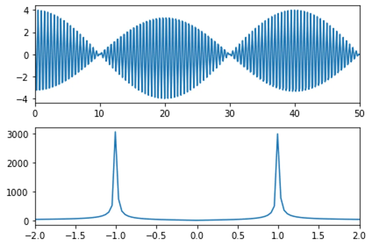
Important: For spectrum, the choice of \(t\) is crucial, note
t = np.linspace(0, 1000, 10000) below, whereas
t = np.linspace(0, 250, 1000) earlier
Question: Why FFT spectrum of the correlation between \(a^{\dagger},a\) and \(\sigma_x, \sigma_x\) gives you the right frequencies ?
def plotCorrelationSpectrum(t,corre,modifyOmega,xlims):
omega, spectrum = spectrum_correlation_fft(t,corre)
fig, axs = plt.subplots(2, 1)
axs[0].plot(t, np.real(corre))
axs[0].set_xlim(*xlims[0])
axs[1].plot(modifyOmega(omega), np.abs(spectrum))
axs[1].set_xlim(*xlims[1])
fig.tight_layout()
plt.show()
t = np.linspace(0, 1000, 10000)
correC = correlation_2op_2t(H, psi0, tlist=None, taulist=t, c_ops=[],
a_op=aC.dag(), b_op=aC)
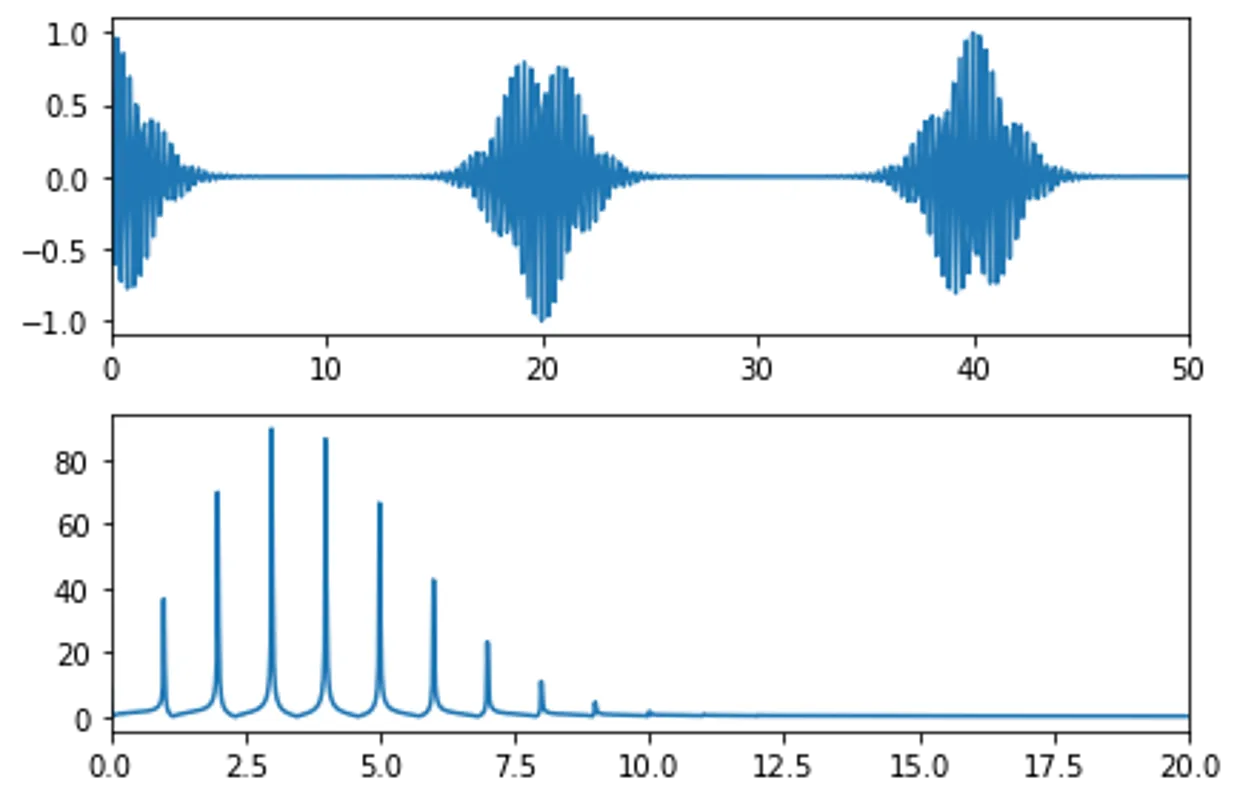
correQ = correlation_2op_2t(H, psi0, tlist=None, taulist=t, c_ops=[],
a_op=XQ.dag(), b_op=XQ) # XQ.dag()=XQ
def modifyOmegaC(omega): return (omega-omegaC)/chi
def modifyOmegaQ(omega): return (omega-omegaQ-chi)/(2*chi)
plotCorrelationSpectrum(t,correC,modifyOmegaC,
xlims=[[0,50],[-2,2]])
plotCorrelationSpectrum(t,correQ,modifyOmegaQ,
xlims=[[0,50],[0,dimC]])
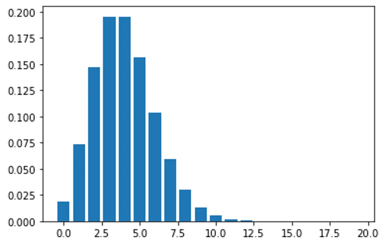
Compare to the cavity fock state distribution:
t = np.linspace(0, 250, 1000)
result = mesolve(H,psi0,t,[],[])
rhoC = ptrace(result.states[-1], 0)
plt.bar(np.arange(0,dimC), np.abs(rhoC.diag()))

rhoList = list(map(getRhoCavity,np.arange(0,250,20)))
plotWigner(rhoList)

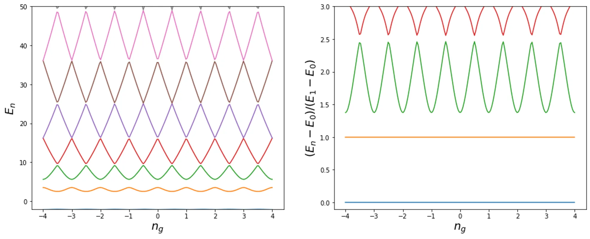
Superconducting charge qubits
Josephson charge qubit:
\[\displaystyle H = \sum_n 4 E_C (n_g - n)^2 \left|n\right\rangle\left\langle n\right| - \frac{1}{2}E_J\sum_n\left(\left|n+1\right\rangle\left\langle n\right| + \left|n\right\rangle\left\langle n+1\right| \right)\]\(E_C\) : Charge energy
\(E_J\) : Josephson energy
\(\left| n\right\rangle\) : the charge state with \(n\) Cooper-pairs on the island that makes up the charge qubit
\(n_g\) : gate bias
Schoelkopf: J. Koch et al, Phys. Rec. A 76, 042319 (2007)
def Hcq(Ec,Ej,N,ng):
    n = np.arange(-N,N+1)
    return Qobj( np.diag(4*Ec*(ng-n)**2) \
                 + 0.5*Ej*np.diag(-np.ones(2*N), 1) \
                 + 0.5*Ej*np.diag(-np.ones(2*N),-1) )

def plotHcqEnergies(ngVec,energies,ymaxs=(50,3)):
    fig, axes = plt.subplots(1,2, figsize=[16,6])
    for n in range( len(energies[0,:]) ) :
        axes[0].plot(ngVec, energies[:,n])
    axes[0].set_ylim(-2, ymaxs[0])
    axes[0].set_xlabel(r'$n_g$', fontsize=18)
    axes[0].set_ylabel(r'$E_n$', fontsize=18)

    for n in range( len(energies[0,:]) ):
        axes[1].plot(ngVec, (energies[:,n]-energies[:,0])/(energies[:,1]-energies[:,0]))
    axes[1].set_ylim(-0.1, ymaxs[1])
    axes[1].set_xlabel(r'$n_g$', fontsize=18)
    axes[1].set_ylabel(r'$(E_n-E_0)/(E_1-E_0)$', fontsize=18)
    plt.show()


N = 10
ngVec = np.linspace(-4, 4, 200)
#Charge qubit regime
Ec = 1.0; Ej = 1.0
energies = np.array([Hcq(Ec, Ej, N, ng).eigenenergies() for ng in ngVec])
#plotHcqEnergies(ngVec, energies)

#Intermediate regime
Ec = 1.0; Ej = 5.0
energies = np.array([Hcq(Ec, Ej, N, ng).eigenenergies() for ng in ngVec])
plotHcqEnergies(ngVec, energies)

#Transmon regime
Ec = 1.0; Ej = 50.0
energies = np.array([Hcq(Ec, Ej, N, ng).eigenenergies() for ng in ngVec])
plotHcqEnergies(ngVec, energies)
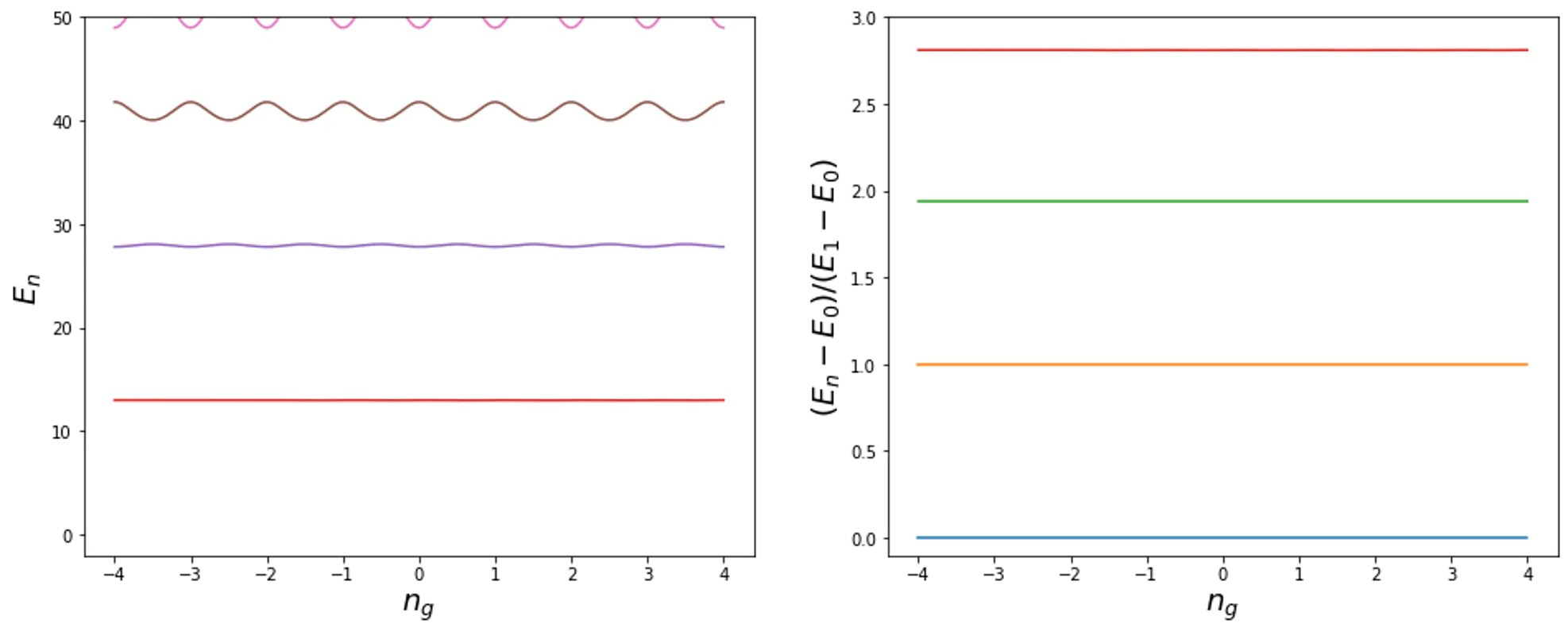
Transmon: - Energy splitting almost independent of the gate bias \(n_g\), thus insensitive to charge noise - But states are not well separated
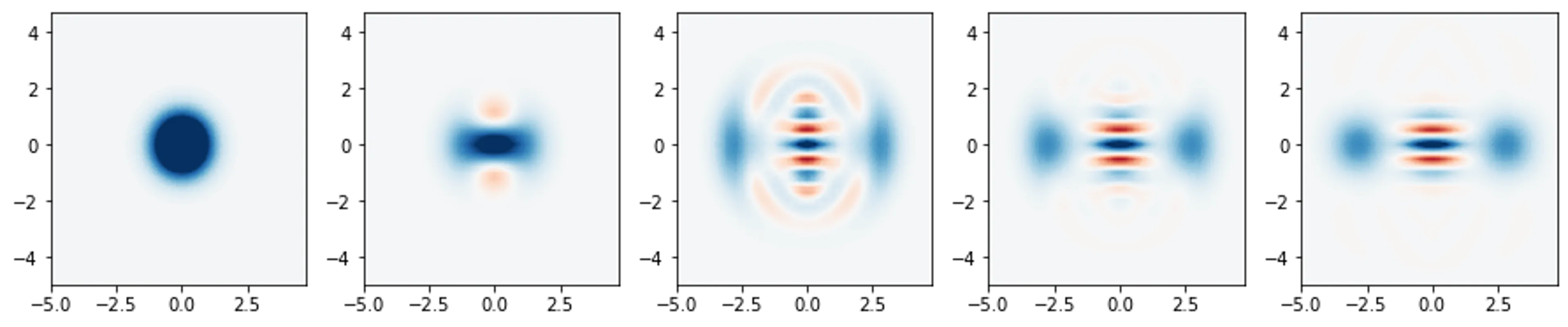
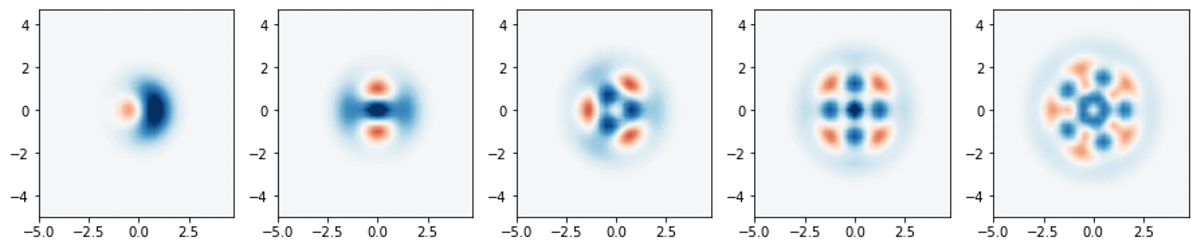
Gallery of Wigner functions
# Superposition of coherent states
alpha = 2
def dimCtoRho(dimC):
psis = [coherent(dimC,-alpha), coherent(dimC,alpha)]
return ket2dm( sum(psis).unit() )
rhoList = list(map(dimCtoRho,range(1,15,3)))
plotWigner(rhoList)
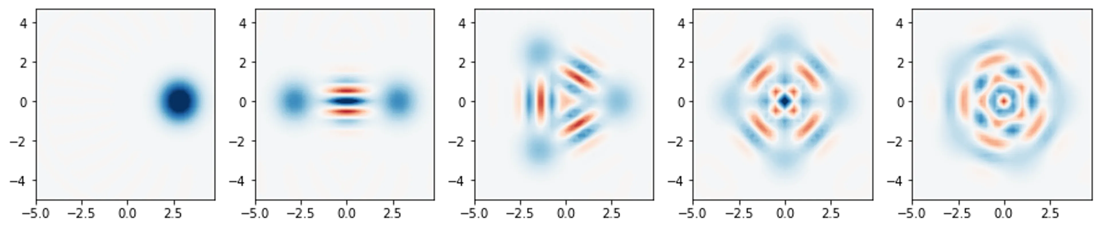
dimC = 20
def MtoRho(M):
psis = [coherent(dimC,2*np.exp(2j*np.pi*m/M)) for m in range(M)]
return ket2dm( sum(psis).unit() )
rhoList = list(map(MtoRho,range(1,6)))
plotWigner(rhoList)
#Superposition of Fock states
dimC = 20
def MtoRho(M):
psis = [fock(dimC,0),fock(dimC,M)]
return ket2dm( sum(psis).unit() )
rhoList = list(map(MtoRho,range(1,6)))
plotWigner(rhoList)
Optimal control - Overview
GRAPE (2005)
Steepest ascent: First order gradient method
- The second order differentials (Hessian matrix) can be used to approximate the local
landscape to a parabola. This way a step (or jump) can be made to where the minima would be if it were parabolic. This typically vastly reduces the number of iterations, and removes the need to guess a step size.
Newton-Raphson method: all elements of the Hessian are calculated
Hessian is expensive
Quasi-Newton: Approximates the Hessian based on successive iterations
Broyden–Fletcher–Goldfarb–Shanno algorithm (BFGS):
scipy.optimize.minimize(fun, x0, args=(), method='L-BFGS-B'),
Limited memory (doesn’t store the entire Hessian) and Bounded (set
bounds for
variables)
- Catch: It is more efficient if the gradients can be calculated
exactly - Closed systems with unitary dynamics - a method using the
eigendecomposition is used - efficient as it is also used in the
propagator calculation (to exponentiate the combined Hamiltonian) - Open
systems and symplectic dynamics - Frechet derivative (or augmented
matrix) method is
used
CRAB (2014) Test result: Slow and inaccurate
Introducing a physically motivated function basis that builds up the pulse
A ‘dressed’ version has recently been introduced that allows to escape local minima
Takes the time evolution as a black-box where the pulse goes as an input and the cost (e.g. infidelity) value will be returned as an output
Optimal control - Hadamard
Drift is \(\sigma_z\) (rotation about \(z\))
Control is \(\sigma_x\) (rotation about \(x\))
Fully controllable: Any unitary target could be chosen
dtmust be chosen such that it is small compared with the dynamics of the systemL-BFGS-B algorithm
At each iteration the gradient of the fidelity error w.r.t. each control amplitude in each timeslot is calculated using an exact gradient method
Using the gradients the algorithm will determine a set of piecewise control amplitudes that reduce the fidelity error
With repeated iterations an approximation of the Hessian matrix is calculated, which enables a quasi 2nd order Newton method for finding a minima
The majority of time is spent calculating the propagators, i.e. exponentiating the combined Hamiltonian
from qutip.qip.operations import hadamard_transform
import qutip.control.pulseoptim as cpo
import datetime
Hd = sigmaz()
Hcs = [sigmax()]
U0 = qeye(2)
Utarg = hadamard_transform(1)
Nt = 10
T = 10

result = cpo.optimize_pulse_unitary(Hd,Hcs,U0,Utarg,Nt,T)

def printOptimizeResult(result,name,U=False):
    if(U): print("Final evolution\n{}\n".format(result.evo_full_final))
    print('*'*20 +' '+ name + " Summary " + '*'*20)
    print("Final fidelity error {}".format(result.fid_err))
    print("Final gradient normal {}".format(result.grad_norm_final))
    print("Terminated due to {}".format(result.termination_reason))
    print("Number of iterations {}".format(result.num_iter))
    print("Completed in {} HH:MM:SS.US".format(
        datetime.timedelta(seconds=result.wall_time)))
printOptimizeResult(result,'Hadamard')
**************** Hadamard Summary ****************
Final fidelity error 9.25592935629993e-13
Final gradient normal 2.4684918139413004e-05
Terminated due to Goal achieved
Number of iterations 4
Completed in 0:00:00.018038 HH:MM:SS.US
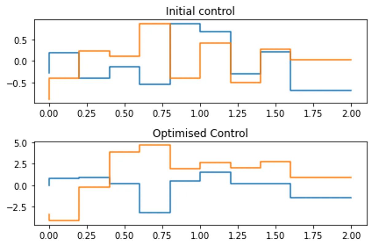
def plotOptimalControl(result):
    fig, axes = plt.subplots(2,1)
    initial = result.initial_amps
    optimised = result.final_amps
    def hstack(x,j): return np.hstack((x[:, j], x[-1, j]))
    for j in range(initial.shape[1]):
        axes[0].step(result.time, hstack(initial,j))
    axes[0].set_title("Initial control")
    for j in range(optimised.shape[1]):
        axes[1].step(result.time, hstack(optimised,j))
    axes[1].set_title("Optimised Control")
    plt.tight_layout()
    plt.show()
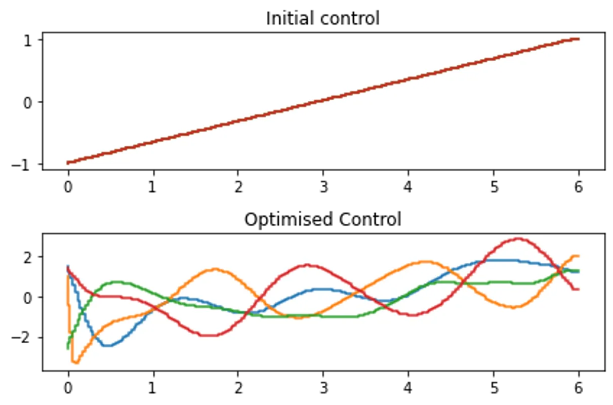
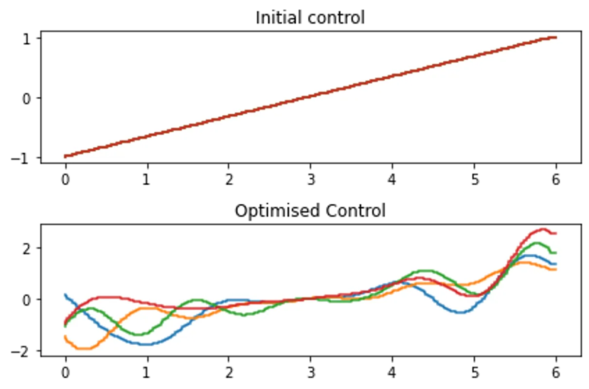
Optimal control - QFT
Two qubits in constant fields in x, y and z
control fields in x and y acting on each qubit
from qutip.qip.algorithms import qft
import qutip.control.pulsegen as pulsegen
X = sigmax(); Y = sigmay(); Z = sigmaz(); I = 0.5*qeye(2)
Hd = 0.5*(tensor(X,X)+tensor(Y,Y)+tensor(Z,Z))
Hcs = [tensor(X,I),tensor(Y,I),tensor(I,X),tensor(I,Y)]
NHcs = len(Hcs)
U0 = qeye(4)
Utarg = qft.qft(2)
Ts = [6]; dt = 0.05
Nt = int(T/dt)

pType = 'LIN'  # gives smooth final pulses

optimizerGRAPE = cpo.create_pulse_optimizer(
    Hd, Hcs, U0, Utarg, Nt, Ts[0], init_pulse_type=pType,
    dyn_type='UNIT', fid_params={'phase_option':'PSU'},
    amp_lbound=-5.0, amp_ubound=5.0,
)
optimizerCRAB = cpo.create_pulse_optimizer(
    Hd, Hcs, U0, Utarg, Nt, Ts[0], init_pulse_type=pType,
    dyn_type='UNIT', fid_params={'phase_option':'PSU'},
    alg='CRAB', prop_type='DIAG', fid_type='UNIT',
    max_iter = 20000,
)

def runOptimizerGRAPE(optimizer):
    dynamics = optimizer.dynamics
    results = []
    for i,T in enumerate(Ts):
        dynamics.init_timeslots()
        pulseGen = pulsegen.create_pulse_gen(pType, dynamics)
        initAmps = np.zeros([dynamics.num_tslots, NHcs])
        for j in range(dynamics.num_ctrls):
            initAmps[:, j] = pulseGen.gen_pulse()
        dynamics.initialize_controls(initAmps)
        result = optimizer.run_optimization()
        printOptimizeResult(result,optimizer.alg+' T = {}'.format(T))
        plotOptimalControl(result)
        results.append(result)
        if i+1 < len(Ts): # reconfigure the dynamics
            dynamics.tau = None
            dynamics.evo_time = Ts[i+1]
            dynamics.num_tslots = int(Ts[i+1]/dt)

def runOptimizerCRAB(optimizer):
    dynamics = optimizer.dynamics
    for i,pulseGen in enumerate(optimizer.pulse_generator):
        guessGen = pulsegen.create_pulse_gen('LIN',dyn=dynamics)
        pulseGen.guess_pulse = guessGen.gen_pulse()
        pulseGen.scaling = 0.0
        pulseGen.num_coeffs = 5
    initAmps = np.zeros([dynamics.num_tslots,dynamics.num_ctrls])
    for j in range(dynamics.num_ctrls):
        pulseGen = optimizer.pulse_generator[j]
        pulseGen.init_pulse()
        initAmps[:, j] = pulseGen.gen_pulse()
    dynamics.initialize_controls(initAmps)
    result = optimizer.run_optimization()
    printOptimizeResult(result,optimizer.alg+' T = {}'.format(Ts[0]))
    plotOptimalControl(result)

runOptimizerGRAPE(optimizerGRAPE)
runOptimizerCRAB(optimizerCRAB)
**************** GRAPE T = 6 Summary ****************
Final fidelity error 4.697306987822003e-10
Final gradient normal 3.793240279665759e-06
Terminated due to function converged
Number of iterations 30
Completed in 0:00:01.396245 HH:MM:SS.US
**************** CRAB T = 6 Summary ****************
Final fidelity error 0.4187122771868691
Final gradient normal 0.0
Terminated due to Max wall time exceeded
Number of iterations 5477
Completed in 0:03:00.013547 HH:MM:SS.US
Optimal control - Lindbladian
Open system
Single qubit subject to an amplitude damping channel
Target evolution: Hadamard gate
For a \(d\) dimensional quantum system in general we represent the Lindbladian as a \(d^2 \times d^2\) dimensional matrix by creating the Liouvillian superoperator
Control generators acting on the qubit are also converted to superoperators
The initial and target maps also need to be in superoperator form
sprepost(A, B)Superoperator formed from pre-multiplication by operator A and post- multiplication of operator B.
from qutip.superoperator import liouvillian, sprepost
X = sigmax(); Y = sigmay(); Z = sigmaz(); I = qeye(2)
sM = sigmam()
hadamard = hadamard_transform(1)

tunnelling = 0.1
omegaQ = 1
Hd = 0.5*omegaQ*sigmaz() + 0.5*tunnelling*X
damping = np.sqrt(0.1)
Ld = liouvillian(Hd, [damping*sM])
Lcs = [liouvillian(Z), liouvillian(X)]
NLcs = len(Lcs)

E0 = sprepost(I, I)
Etarg = sprepost(hadamard, hadamard)

Nt = 10; T = 2

result = cpo.optimize_pulse(Ld, Lcs, E0, Etarg, Nt, T)
printOptimizeResult(result,'Lindbladian')
plotOptimalControl(result)
**************** Lindbladian Summary ****************
Final fidelity error 0.005845509986664133
Final gradient normal 9.438858417223121e-06
Terminated due to function converged
Number of iterations 167
Completed in 0:00:01.718335 HH:MM:SS.US