CODE 1D DFT
Note
The .rst file for this page is generated using Jupyter Notebook, from the .ipynb file: Density Functional Theory 1D
Credit
This note is modified from Numpy 1D-DFT
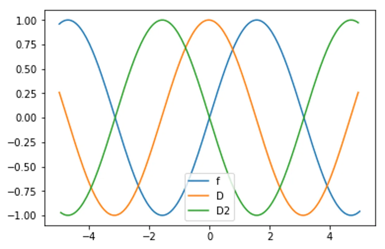
Differentiation
First order differentiation
Second order differentiation
import numpy as np
import matplotlib.pyplot as plt

n_grid=200
x=np.linspace(-5,5,n_grid)
y=np.sin(x)

Delta_x = x[1] - x[0]
print(np.diagflat(np.ones(n_grid-1),-2))
print(np.eye(n_grid))
D = np.diagflat(np.ones(n_grid-1),1) - np.eye(n_grid)
D = D / Delta_x

D2 = - D.dot(D.T)
D2[-1,-1]=D2[0,0] #The derivative may not be well defined at the end of the grid

plt.plot(x,y, label="f")
plt.plot(x[:-1],D.dot(y)[:-1], label="D")
plt.plot(x[1:-1],D2.dot(y)[1:-1], label="D2")
plt.legend()
[[0. 0. 0. ... 0. 0. 0.]
 [0. 0. 0. ... 0. 0. 0.]
 [1. 0. 0. ... 0. 0. 0.]
 ...
 [0. 0. 0. ... 0. 0. 0.]
 [0. 0. 0. ... 0. 0. 0.]
 [0. 0. 0. ... 1. 0. 0.]]
[[1. 0. 0. ... 0. 0. 0.]
 [0. 1. 0. ... 0. 0. 0.]
 [0. 0. 1. ... 0. 0. 0.]
 ...
 [0. 0. 0. ... 1. 0. 0.]
 [0. 0. 0. ... 0. 1. 0.]
 [0. 0. 0. ... 0. 0. 1.]]
<matplotlib.legend.Legend at 0x7fcc1fc68048>
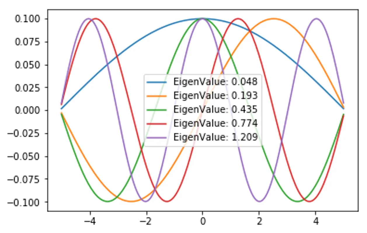
Free particle Hamiltonian
(in a box given by grid size 10)
hbar = 1
m = 1
H_FreeParticle = - (hbar**2/(2*m)) * D2
EigenValue, EigenVector_FreeParticle = np.linalg.eigh(H_FreeParticle)

for i in range(5):
  plt.plot(x,EigenVector_FreeParticle[:,i], label=f"EigenValue: {EigenValue[i]:.3f}")
plt.legend()
<matplotlib.legend.Legend at 0x7fcc22da2da0>
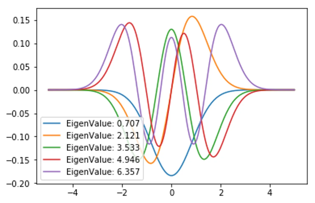
Harmonic oscillator
HarmonicPotential = np.diagflat(x*x)
H_HarmonicOscillator = H_FreeParticle + HarmonicPotential
EigenValue, EigenVector_HarmonicOscillator = np.linalg.eigh(H_HarmonicOscillator)

for i in range(5):
  plt.plot(x,EigenVector_HarmonicOscillator[:,i], label=f"EigenValue: {EigenValue[i]:.3f}")
plt.legend()
<matplotlib.legend.Legend at 0x7fcc22480358>
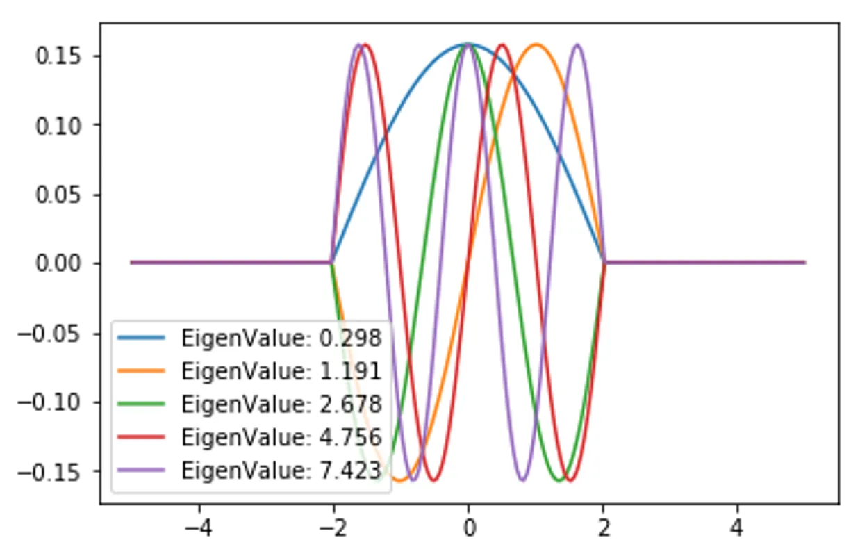
Potential well
PotentialWell = np.full_like(x,1e10)
PotentialWell[np.logical_and(x>-2,x<2)] = 0
PotentialWell = np.diagflat(PotentialWell)

H_PotentialWell = H_FreeParticle + PotentialWell
EigenValue, EigenVector_PotentialWell = np.linalg.eigh(H_PotentialWell)

for i in range(5):
  plt.plot(x,EigenVector_PotentialWell[:,i], label=f"EigenValue: {EigenValue[i]:.3f}")
plt.legend()
<matplotlib.legend.Legend at 0x7fcc1fae82e8>
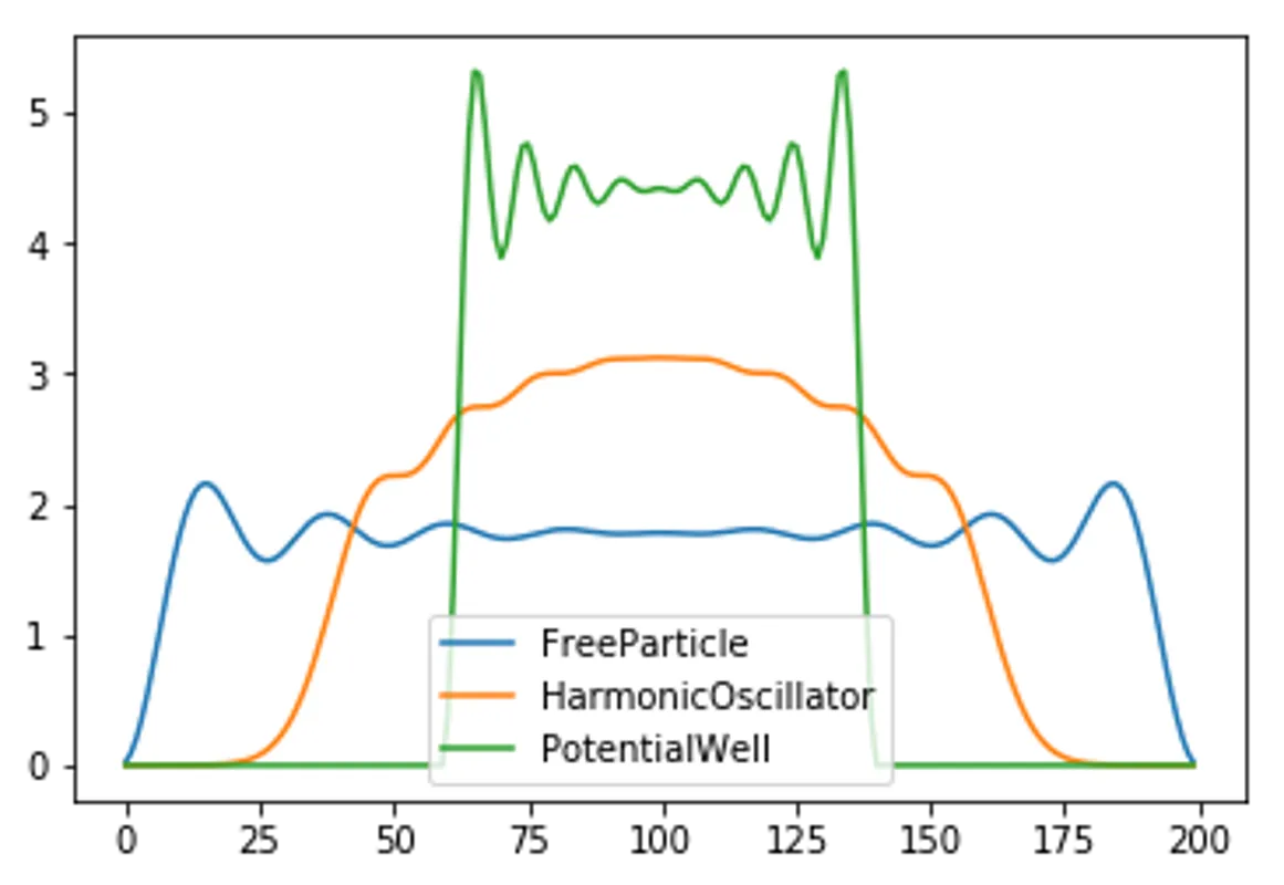
Density
Each state \(k\) (EigenVector) can have \(N_k=0,1\text{ or }2\) electrons
Note that the eigenvalues (energy) given by np.linalg.eigh is automatically ordered from small to large
Thus if \(N_\text{total}=5\) for example, \(N_0=N_1=2,N_2=1,N_{>2}=0\)
def Integrate(x,y,axis = 0):
  dx = x[1]-x[0]
  return np.sum(y*dx, axis = axis)


def GetDensity(N_total, psi, x):
  I = Integrate(x,psi**2)
  normalized_psi = psi/np.sqrt(I)[None,:]  # ???

  N_k = [2 for _ in range(N_total//2)]
  if N_total % 2:
    N_k.append(1)

  density = np.zeros_like(normalized_psi[:,0])
  for N_k_, psi in zip(N_k, normalized_psi.T):
    density += N_k_ * (psi**2)
  return density

N_total = 17
plt.plot(GetDensity(N_total,EigenVector_FreeParticle, x), label="FreeParticle")
plt.plot(GetDensity(N_total,EigenVector_HarmonicOscillator, x), label="HarmonicOscillator")
plt.plot(GetDensity(N_total,EigenVector_PotentialWell, x), label="PotentialWell")
plt.legend()
<matplotlib.legend.Legend at 0x7fcc1fa1f240>
Functional Derivative
a generalization of the Euler–Lagrange equation:
Exchange Potential
The Exchange-Correlation Functional is a correction to the electronic energy that approximates the effect of electron interactions.
To keep life simple, we ignore Correlation because its expression is more tedious than interesting to implement.
Consider therefore the Exchange Functional in the Local Density Approximation (LDA):
In the derivation of the Kohn-Sham Equations, the potential corresponding to each energy term is defined as the derivative of the energy with respect to the density. The Exchange Potential is therefore:
def GetExchange(n,x):
  ExchangeEnergy = -3/4 * (3/np.pi)**(1/3) * Integrate(x, n**(4/3))
  ExchangePotential = - (3/np.pi)**(1/3) * n**(1/3)
  return ExchangeEnergy, ExchangePotential
Coulomb potential
The Electrostatic Energy or Hartree Energy is given by
This expression converges in 3D, but not in 1D. Hence we cheat and use a modified form:
Again, the potential is the derivative of the energy with respect to the density:
def GetHartree(n,x,epsilon=1e-1):
  Delta_x = x[1]-x[0]
  HartreeEnergy = 1/2*np.sum(n[None,:]*n[:,None]/np.sqrt((x[None,:]-x[:,None])**2+epsilon)*Delta_x*Delta_x)
  HartreePotential = np.sum(n[None,:]/np.sqrt((x[None,:]-x[:,None])**2+epsilon)*Delta_x, axis=-1)
  return HartreeEnergy, HartreePotential
Solve the Kohn–Sham Equations: Self-Consistency Loop
initialize the density (you can take an arbitrary constant)
Calculate the Exchange and Hatree potentials
Calculate the Hamiltonian
Calculate the eigenvalues and eigenvectors (wavefunctions)
If not converged, calculate the density and back to 1
n = np.zeros(n_grid)
LastEnergy = float("inf")
for i in range(1000):
ExchangeEnergy, ExchangePotential = GetExchange(n,x)
HartreeEnergy, HartreePotential = GetHartree(n,x)
H = H_FreeParticle + HarmonicPotential + np.diagflat(ExchangePotential+HartreePotential)
EigenValue, EigenVector_DFT = np.linalg.eigh(H)
change = abs(EigenValue[0]-LastEnergy)
LastEnergy = EigenValue[0]
print("Ground State Energy:",EigenValue[0],".. Change:",change)
if change < 1e-5:
break
n = GetDensity(N_total, EigenVector_DFT, x)
'''
for i in range(5):
plt.plot(x,EigenVector_DFT[:,i], label=f"EigenValue: {EigenValue[i]:.3f}")
plt.legend()
'''
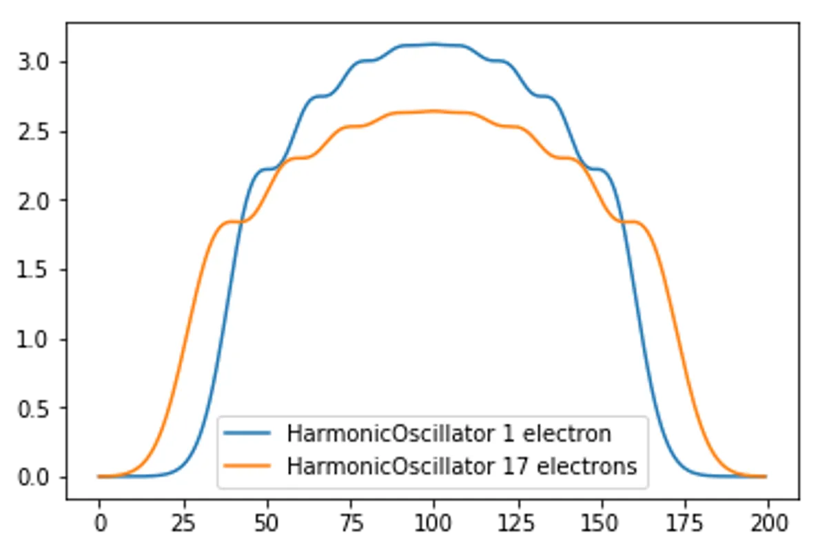
plt.plot(GetDensity(N_total,EigenVector_HarmonicOscillator, x), label="HarmonicOscillator 1 electron")
plt.plot(GetDensity(N_total, EigenVector_DFT, x), label="HarmonicOscillator 17 electrons")
plt.legend()
Ground State Energy: 0.7069489216396394 .. Change: inf
Ground State Energy: 16.362481113553386 .. Change: 15.655532191913746
Ground State Energy: 13.802125164165675 .. Change: 2.560355949387711
Ground State Energy: 15.300177750512375 .. Change: 1.4980525863467005
Ground State Energy: 14.411948982556314 .. Change: 0.8882287679560612
Ground State Energy: 14.946992808765927 .. Change: 0.5350438262096127
Ground State Energy: 14.624165620778795 .. Change: 0.32282718798713184
Ground State Energy: 14.820098486380779 .. Change: 0.19593286560198386
Ground State Energy: 14.701062940689484 .. Change: 0.11903554569129504
Ground State Energy: 14.773528046467316 .. Change: 0.07246510577783205
Ground State Energy: 14.729396772844979 .. Change: 0.044131273622337375
Ground State Energy: 14.756291444171477 .. Change: 0.02689467132649881
Ground State Energy: 14.739899203648717 .. Change: 0.01639224052276056
Ground State Energy: 14.749892601933313 .. Change: 0.009993398284596111
Ground State Energy: 14.743800001840365 .. Change: 0.00609260009294843
Ground State Energy: 14.747514729729723 .. Change: 0.003714727889358116
Ground State Energy: 14.745249799055264 .. Change: 0.002264930674458654
Ground State Energy: 14.746630802141052 .. Change: 0.001381003085787924
Ground State Energy: 14.745788757575497 .. Change: 0.0008420445655552555
Ground State Energy: 14.746302185556894 .. Change: 0.0005134279813976406
Ground State Energy: 14.745989128109859 .. Change: 0.00031305744703580274
Ground State Energy: 14.746180012284182 .. Change: 0.00019088417432300275
Ground State Energy: 14.746063622259712 .. Change: 0.00011639002446983682
Ground State Energy: 14.746134590178523 .. Change: 7.096791881089359e-05
Ground State Energy: 14.746091318041849 .. Change: 4.3272136673877526e-05
Ground State Energy: 14.746117702900854 .. Change: 2.638485900519072e-05
Ground State Energy: 14.746101614932831 .. Change: 1.6087968022659993e-05
Ground State Energy: 14.746111424450689 .. Change: 9.8095178575619e-06
<matplotlib.legend.Legend at 0x7fcc1f998f60>
Wrap up
import numpy as np
import matplotlib.pyplot as plt
def Integrate(x,y,axis = 0):
dx = x[1] - x[0]
return np.sum(y*dx, axis = axis)
def GetDensity(N_total, psi, x):
I = Integrate(x,psi**2)
normalized_psi = psi/np.sqrt(I)[None,:]
N_k = [2 for _ in range(N_total//2)]
if N_total % 2:
N_k.append(1)
n = np.zeros_like(normalized_psi[:,0])
for N_k_, psi in zip(N_k, normalized_psi.T):
n += N_k_ * (psi**2)
return n
def GetExchange(n,x):
ExchangeEnergy = -3/4 * (3/np.pi)**(1/3) * Integrate(x, n**(4/3))
ExchangePotential = - (3/np.pi)**(1/3) * n**(1/3)
return ExchangeEnergy, ExchangePotential
def GetHartree(n,x,epsilon=1e-1):
dx = x[1]-x[0]
HartreeEnergy = 1/2*np.sum(n[None,:]*n[:,None]/np.sqrt((x[None,:]-x[:,None])**2+epsilon)*dx*dx)
HartreePotential = np.sum(n[None,:]/np.sqrt((x[None,:]-x[:,None])**2+epsilon)*dx, axis=-1)
return HartreeEnergy, HartreePotential
class SimpleDFT:
def __init__(self, N_total=17, x_begin=-5, x_end=5, n_grid = 200,
hbar = 1, m = 1):
self.n_grid = n_grid
self.N_total = N_total
self.x = np.linspace(x_begin,x_end,n_grid)
self.dx = self.x[1] - self.x[0]
self.D = np.diagflat(np.ones(n_grid-1),1) - np.eye(n_grid)
self.D = self.D / self.dx
self.D2 = - self.D.dot( self.D.T )
self.D2[-1,-1] = self.D2[0,0] #The derivative may not be well defined at the end of the grid
self.H_FreeParticle = - (hbar**2/(2*m)) * self.D2
def FreeParticle(self):
Potential = 0
self.Solve("FreeParticle",Potential)
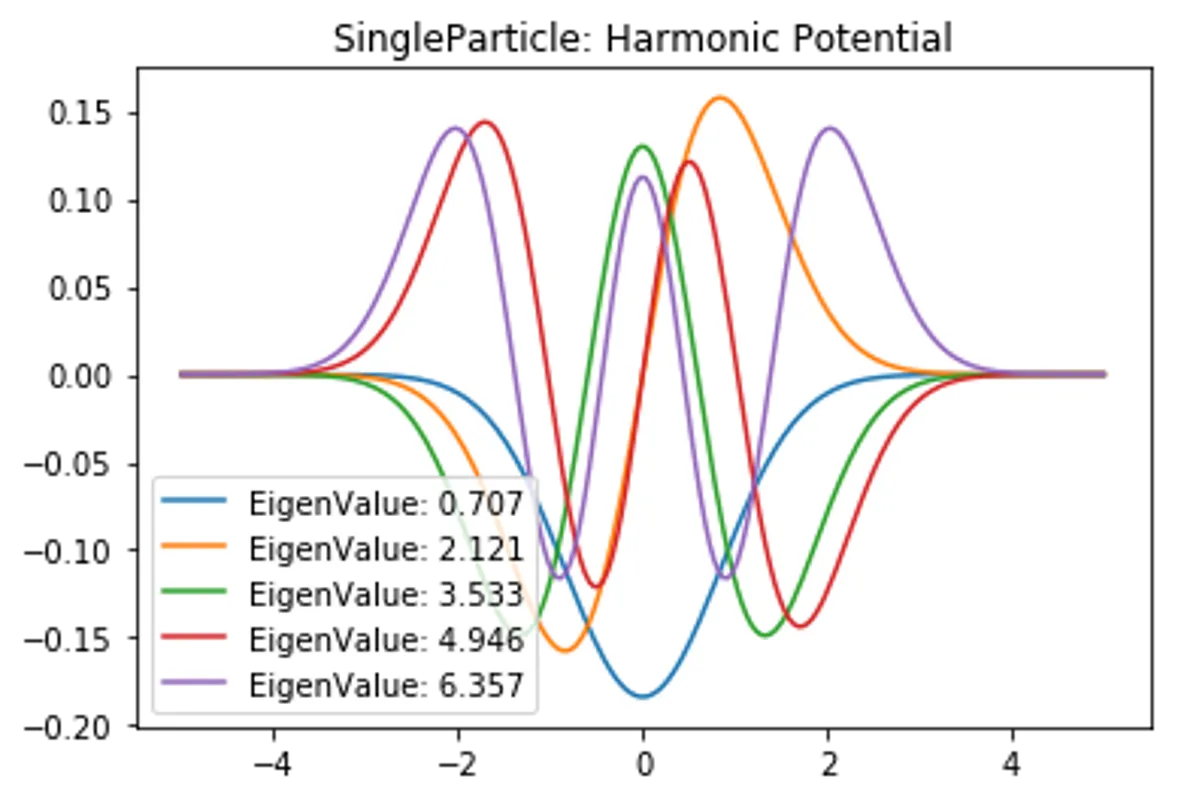
def HarmonicPotential(self,k=1):
Potential = np.diagflat(k * self.x*self.x)
self.Solve("Harmonic Potential", Potential)
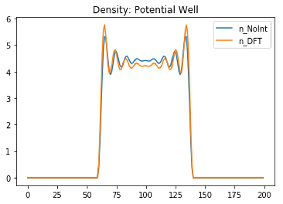
def PotentialWell(self, width = 4,center =0):
Potential = np.full_like(self.x,1e10)
Potential[np.logical_and(self.x> center-width/2, self.x< center+width/2)] = 0
Potential = np.diagflat(Potential)
self.Solve("Potential Well", Potential)
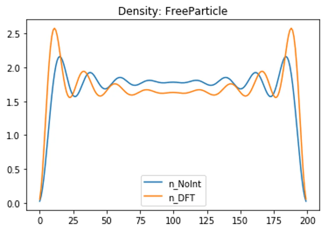
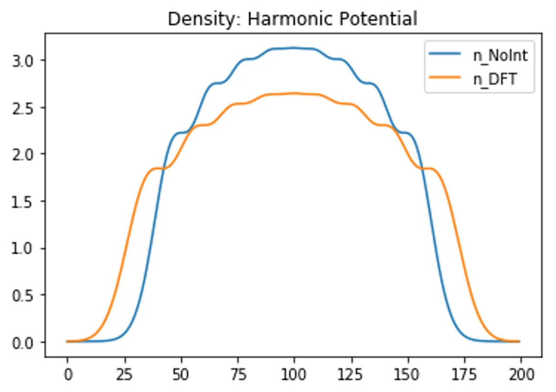
def Solve(self,PotentialName, Potential):
_,_,n_NoInt = self.SolveSingleParticle( PotentialName, Potential)
_,_,n_DFT = self.SolveManyParticle( PotentialName, Potential)
plt.title("Density: "+PotentialName)
plt.plot(n_NoInt,label="n_NoInt"), plt.plot(n_DFT,label="n_DFT")
plt.legend(), plt.show()
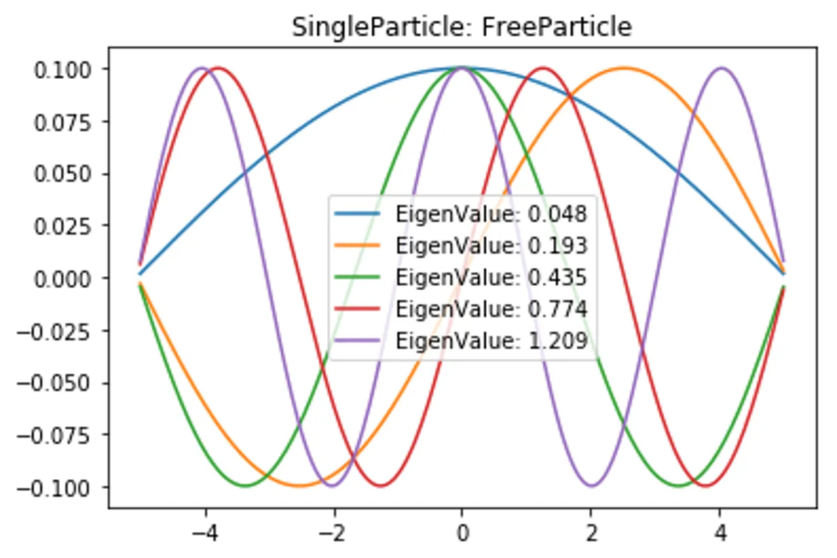
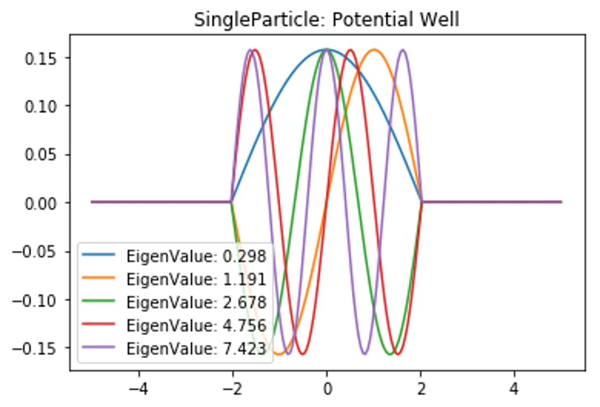
def SolveSingleParticle(self,PotentialName, Potential):
H = self.H_FreeParticle + Potential
EigenValue, EigenVector = np.linalg.eigh(H)
n = GetDensity(self.N_total, EigenVector, self.x)
plt.title("SingleParticle: "+PotentialName)
for i in range(5):
plt.plot(self.x,EigenVector[:,i], label=f"EigenValue: {EigenValue[i]:.3f}")
plt.legend(), plt.show()
return EigenValue, EigenVector, n
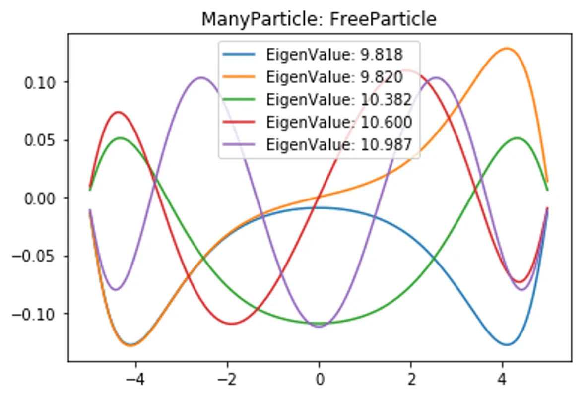
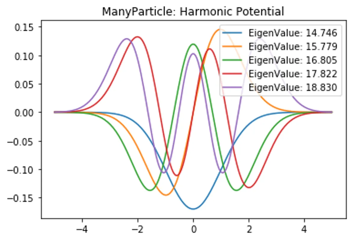
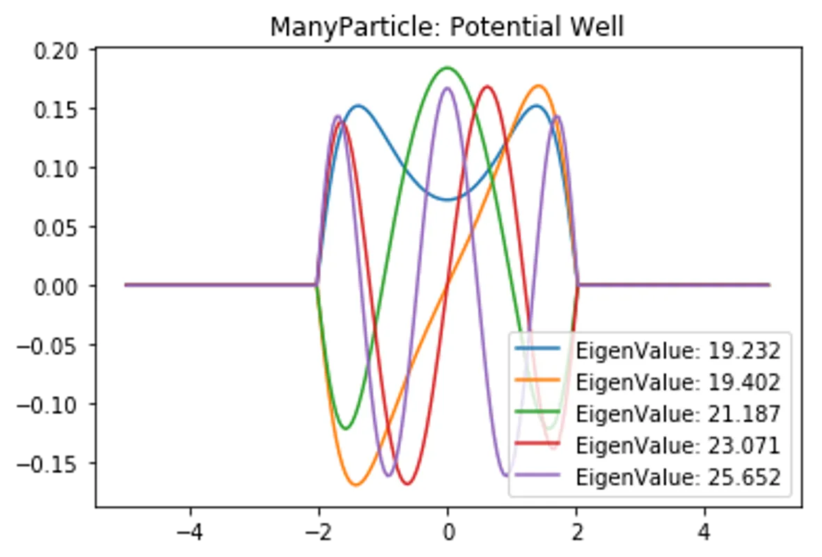
def SolveManyParticle(self, PotentialName, Potential):
n = np.zeros(self.n_grid)
LastEnergy = float("inf")
for i in range(1000):
ExchangeEnergy, ExchangePotential = GetExchange(n,self.x)
HartreeEnergy, HartreePotential = GetHartree(n,self.x)
H = self.H_FreeParticle + Potential + np.diagflat(ExchangePotential+HartreePotential)
EigenValue, EigenVector = np.linalg.eigh(H)
change = abs(EigenValue[0]-LastEnergy)
LastEnergy = EigenValue[0]
#print("Ground State Energy:",EigenValue[0],".. Change:",change)
if change < 1e-5:
break
n = GetDensity(self.N_total, EigenVector, self.x)
plt.title("ManyParticle: "+PotentialName)
for i in range(5):
plt.plot(self.x,EigenVector[:,i], label=f"EigenValue: {EigenValue[i]:.3f}")
plt.legend(), plt.show()
return EigenValue, EigenVector, n
# usage
SimpleDFT_1 = SimpleDFT()
SimpleDFT_1.FreeParticle()
SimpleDFT_1.HarmonicPotential()
SimpleDFT_1.PotentialWell()