CODE 1D DPFT

Date:: 8 Oct 2019

Note

The .rst file for this page is generated using Jupyter Notebook, from the .ipynb file: 1D DPFT In Python

Thomas Fermi Kinetic Energy

\[\begin{split}E_{\text{kin}}=\int dx\; {1\over 3}\alpha \bar{n}^3 \\ \Rightarrow {\delta E_{\text{kin}} \over \delta n}=\alpha n^2\end{split}\]

Where \(\alpha \equiv {\pi^2\hbar^2\over 2mg^2}\)

And \(g\) is spin multiplicity. For spin-polarized fermi gas (For example electron gas with all the electrons spin-up), \(g=1\) from Pauli principle

Without Interaction

\[\begin{split}\begin{cases} \delta\left(E_{\text{kin}}+E_{\text{ext}}\right)=0 \\ {\delta E_{\text{ext}} \over \delta n}= V_{\text{ext}} - \mu \end{cases} \\ \Rightarrow n_{\text{nonInt}}[\mu-V_{\text{ext}}]=\sqrt{\alpha^{-1}[\mu-V_{\text{ext}}]_+}\end{split}\]

is a Functional of \(\mu-V_{\text{ext}}\)

Where \(\mu\) is the chemical potential

The Interaction

\[\begin{split}E_{\text{int}} = w{1\over 2}\int{dr\; n^2(r)} \\ \Rightarrow V_{\text{int}}={\delta E_{\text{int}} \over \delta n}=wn\end{split}\]

Where \(w\) is strength of interaction
Then we have

\[\begin{split}\delta\left(E_{\text{kin}}+E_{\text{ext}}+E_{\text{int}} \right)=0 \\ \Rightarrow n_{\text{int}}(x,\mu)=\left(-{w\over 2\alpha}+\sqrt{ ( {w\over 2\alpha})^2 +{\mu-V_{\text{ext}} \over \alpha} }\right) \eta(\mu-V_{\text{ext}})\end{split}\]

Self Consistent Loop

What is the idea?

We will find \(n\) with interaction
However, we will NOT use the expression \(n_{\text{int}}\) above
Instead, we use the expression \(n_{\text{nonInt}}\):
1. Specifically we will use \(n=\sqrt{\alpha^{-1}[\mu-V]_+}\)
2. We initialize \(V\) with \(V_{\text{ext}}\)
3. Then we find the chemical potential \(\mu\) using gradient descent, the loss function would be \(N-\int n(x) \;dx\), we do this to make sure the total particle number is constant
4. Then we calculate \(n_{\text{modified}}\) based on \(\mu\) and \(V\) using above formula
5. Then we update \(n\) by mixing the old \(n\) with \(n_{\text{modified}}\), that is \(n=(1-p)n+p\; n_{\text{modified}}\), the idea is similar to gradient descent, the \(p\) here can be understood as learning rate
6. Using the new \(n\) we can calculate \(V_{\text{int}}=wn\), then we add the interaction energy to \(V_{\text{ext}}\) as our modified \(V\), that is \(V=V_{\text{ext}}+V_{\text{int}}\)
7. Then we can go back to \(3\) until \(n\) converges

Simple implementation in Python

import numpy as np
import matplotlib.pyplot as plt

class SimpleDPFT:
  def __init__(self,args):
    self.Vext = args["Vext"]
    self.maxIteration = args["maxIteration"]
    self.mu = args["mu"]
    self.alpha = args["alpha"]
    self.N = args["N"]
    self.dx = args["dx"]
    self.learningRate = args["learningRate"]
    self.gradientMax = args["gradientMax"]
    self.w = args["w"]
    self.p = args["p"]
    self.nChangeMax = args["nChangeMax"]

  def selfConsistentLoop(self):
    self.V = self.Vext
    self.mu = self.enforceN(self.mu)
    self.n = self.getDensity(self.mu)
    for i in range(self.maxIteration):
      self.V = self.Vext + self.w * self.n
      self.mu = self.enforceN(self.mu)
      nOld = self.n
      self.n = (1-self.p)*self.n + self.p*self.getDensity(self.mu)
      if(np.sum(abs(self.n-nOld))<self.nChangeMax):
        break
    return self.n

  def enforceN(self, mu):
    # gradient descent
    for i in range(self.maxIteration):
      gradient = (self.cost(mu+1)-self.cost(mu))
      mu = mu - self.learningRate * gradient
      if(abs(gradient)<self.gradientMax):
        break
    return mu
  def cost(self, mu):
    return abs(self.N - np.sum(self.getDensity(mu)*self.dx) )

  def getDensity(self,mu):
    muMinusV = mu - self.V
    muMinusV[ muMinusV<0 ] = 0
    return np.sqrt(1/self.alpha * muMinusV)

# =================================================
# ================= Usage =========================
# =================================================
x = np.linspace(-10, 10, num=100)
dx = x[1]-x[0]
args = {
    "Vext": x**2,
    "maxIteration": 4000,
    "mu": 1,
    "alpha": np.pi**2/2,
    "N": 20,
    "dx": dx,
    "learningRate": 1e-1,
    "gradientMax": 1e-6,
    "w": 5,
    "p": 0.5,
    "nChangeMax": 1e-6,
}

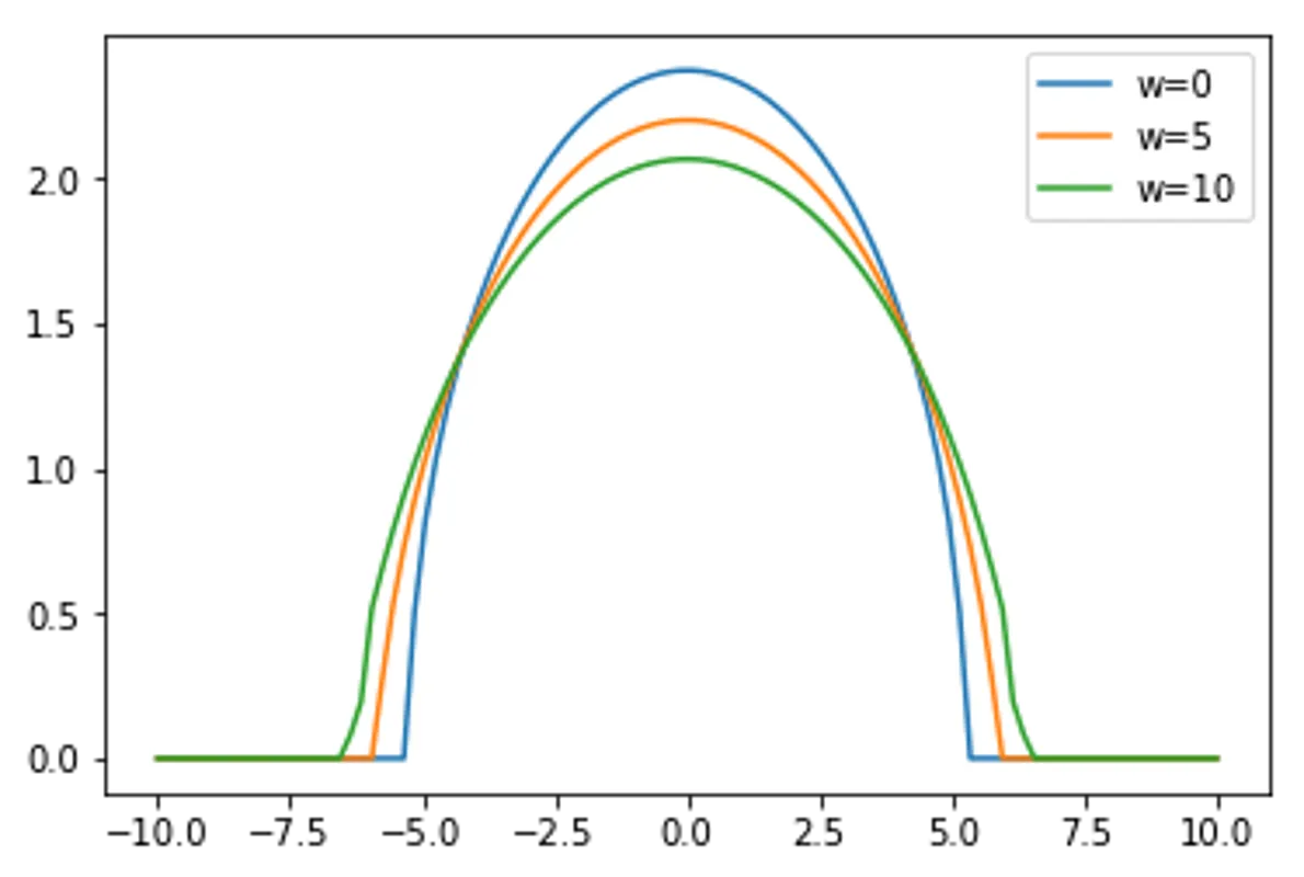
for w in range(3):
  args["w"] = w*5
  simpleDPFT = SimpleDPFT(args)
  n = simpleDPFT.selfConsistentLoop()
  print("Particle Number Check:", np.sum(n)*dx,"/ 20")
  plt.plot(x,n,label="w="+str(w*5))
plt.legend()
plt.show()

Particle Number Check: 19.651993996020014 / 20
Particle Number Check: 19.524746349214976 / 20
Particle Number Check: 19.440909250694254 / 20